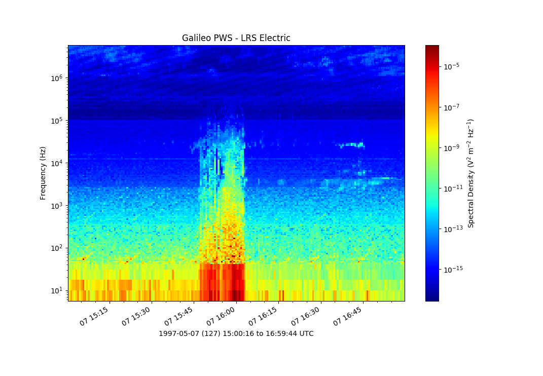
Ex 02: Simple Cubic Spectra
Plotting simple cubic spectra from the Galileo PWI using pcolormesh.

1 2 3 4 5 6 7 8 9 10 11 12 13 14 15 16 17 18 19 20 21 22 23 24 25 26 27 28 29 30 31 32 33 34 35 36 37 38 39 40 41 42 43 44 45 46 47 48 49 50 51 52 53 54 55 56 57 58 59 60 61 62 63 64 65 66 67 68 69 70 71 72 73 74 75 76 77 78 79 80 81 82 83 84 85 86 87 88 | # das2 module example 2:
# Plotting simple cubic Galileo PWS spectra
import das2
import das2.mpl # Extra helpers for interfacing to matplotlib
import matplotlib.pyplot as pyplot
import matplotlib.colors as colors
import matplotlib.dates as dates
# Get a data source definition from the federated catalog system. The ID below
# should not change due to server outages or dataset migration so long as the
# catalog is updated. Each ID can map to mutiple URLs for automatic failover.
# In reality a valid URI is transmitted on the wire, not just the ID below.
# Das2py knows to prepend 'tag:das2.org:2012:' automatically when looking for
# data sources if this prefix is not present.
sId = "site:/uiowa/galileo/pws/survey_electric/das2"
print("Getting data source definition for %s"%sId)
src = das2.get_source(sId)
# Get data from the source. Note, if no parameters are specifed the default
# range and resolution in the source definition will be used
print("Reading default example Galileo PWS E-Survey data...")
lDs = src.get()
ds = lDs[0] # simple example, real code should check dataset list size
print("%d datasets returned"%len(lDs))
# Optionally, print a summary of the dataset
#print(ds)
# The dataset object returned by the data source is a bit more complex than a
# CDF object, but simpler than an HDF database. It was designed to provide
# explicit details regarding the layout and purpose each variable without
# conflating iteration index space with real physical dimensions (though the two
# sets may happen to be related)
time = ds['time'] # These represent real-world physical dimesions.
freq = ds['frequency'] # Dimensions have 1 or more variables (below)
specDens = ds['electric'] # that provide data values.
# das2py Variables provide ndarray views for accessing data. Every Variable
# in the Dataset has the same bulk iteration properites. They have the same
# index ranges for the same index dimensions... always. Said another way,
# Datasets consist of Variables correlated in index space. So:
#
# time['center'][i,j] is the time value for
#
# freq['center'][i,j] is the frequency value for
#
# specDens['center'][i,j].
#
# Always. No matter the internal data storage model.
#
# By providing a single general interface (scatter data), special case handling
# is avoided.
# The pcolormesh plotter from matplotlib works well enough with this data model.
# But a general re-binning plotter should be used instead.
aX = time['center'].array
aY = freq['center'].array
aZ = specDens['center'].array
if specDens.propEq('scaleType','log'):
clrscale = colors.LogNorm(vmin=aZ.min(), vmax=aZ.max())
else:
clrscale = None
(fig, ax0) = pyplot.subplots()
im = ax0.pcolormesh(aX, aY, aZ, norm=clrscale, cmap='jet' )
cbar = fig.colorbar(im, ax=ax0)
if freq.propEq('scaleType','log'):
ax0.set_yscale('log')
fig.autofmt_xdate() # Fix date formating
ax0.fmt_xdata = dates.DateFormatter("%Y-%m-%dT%H:%M") # High-Res in mouse over
ax0.xaxis.set_minor_locator(dates.MinuteLocator(interval=5)) # add minor ticks
# Set plot labels, will use matplotlib helpers from das2 module to format labels
ax0.set_xlabel(das2.mpl.range(time) )
ax0.set_ylabel(das2.mpl.text(freq.props['label']))
cbar.set_label(das2.mpl.text(specDens.props['label']) )
ax0.set_title(das2.mpl.text(ds.props['title']) )
pyplot.show()
|